Guide: Training Your First Linear Regression AI Model with Keras

Introduction

In this guide, you will learn how to create and train a simple linear regression model using Keras (a high-level deep learning library). We'll generate a synthetic dataset, build a neural network, train it, and evaluate its performance. By the end, you'll have a working AI model that predicts values based on input data.

Prerequisites

• Basic understanding of Python
• Familiarity with linear regression (y = mx + b)
• A Google Drive account

Step 2: Import libraries

We will import some important libraries for our use. Libraries are groups of code that simplify many functions for us. Imagine them as rice-cookers: you tell it to cook rice, and specify what rice it is, and it will automatically implement the cooking for you.

import numpy as np  # For math
import matplotlib.pyplot as plt  # To plot our data and results
from tensorflow.keras.models import Sequential  # The framework for our model
from tensorflow.keras.layers import Dense  # One of the components of our model

Step 3: Create Synthetic Data

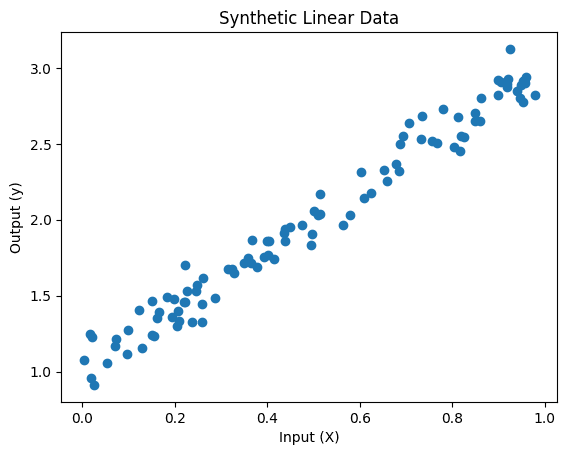
We'll generate data following y = 2x + 1 + noise

# Generate 100 random points
np.random.seed(42)  # For reproducibility
X = np.random.rand(100, 1)
y = 2 * X + 1 + np.random.randn(100, 1) * 0.2  # Added noise

# Visualize
plt.figure(figsize=(8,5))
plt.scatter(X, y, alpha=0.7)
plt.title("Synthetic Linear Dataset")
plt.xlabel("Input Feature (X)")
plt.ylabel("Target Value (y)")
plt.grid(True)
plt.show()

Your visualized data should look something like this. The exact locations of the points may differ due to the random noise added, but it should show a similar trend.

Step 3: Build the Model

Here, we use the Tensorflow Keras library to create our very first single-neuron linear regression neural network model!

Our model only has one "Dense" layer, which is the default neuron structure. Since our dataset is pretty simple, one neuron will do the trick. So we set the number of neurons - "units" to 1. And since our input X is just one number, we set "input_shape" to [1]. (Don't worry about the square bracket yet, it is just how Tensorflow likes its inputs to look.)

# Create a Sequential model
# This is how Tensorflow organizes its models, in a sequence
model = Sequential()

# Add a single Dense (fully connected) layer with 1 neuron
model.add(Dense(1, input_shape=(1,)))

# Compile the model with Mean Squared Error (MSE) loss and Stochastic Gradient Descent (SGD)
# MSE means taking the average of the squared-error between our model's guess and the ground truth
# SGD is a method to "teach" the model how to become more accurate
model.compile(optimizer='sgd', loss='mse')

# Print model summary
model.summary()

It should show us a summary of our model that looks like this

Model: "sequential_1"
_________________________________________________________________
Layer (type)                 Output Shape              Param #   
=================================================================
dense (Dense)                (None, 1)                 2         
=================================================================
Total params: 2
Trainable params: 2
Non-trainable params: 0

Step 4: Train our Model

Finally we let our model try its predictions on our dataset.

This may take a while to run.

# Train the model for 100 epochs (iterations over the dataset)
history = model.fit(X, y, epochs=100, verbose=1)

# Plot training loss over epochs
plt.plot(history.history['loss'])
plt.xlabel("Epochs")
plt.ylabel("Loss (MSE)")
plt.title("Training Loss Over Time")
plt.show()

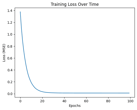
You will also get a plot showing the training loss over time. Loss is a way to measure how inaccurate a model's predictions are.

It usually is not correct in the beginning, hence the high loss. However, our model learns to minimize the loss, or in other words, learn to be correct.

Therefore after a few epochs (rounds of learning), we can see the loss gradually decreasing until our model is reasonable accurate in its predictions.

Step 5: Deploy our Model on New Data

Let's see how well our model works on new data

# Predict y for new X values
X_test = np.array([[0.2], [0.5], [0.8], [1.0]])
y_pred = model.predict(X_test)

print("Predictions:")
for x1, y1 in zip(X_test, y_pred):
    print(f"X = {x1[0]:.2f} → Predicted y = {y1[0]:.2f}")

# Plot predictions vs true data
plt.scatter(X, y, label="True Data")
plt.scatter(X_test, y_pred, label="Predictions")
plt.xlabel("X")
plt.ylabel("y")
plt.legend()
plt.show()

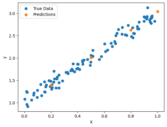
The blue dots are our training data, and the orange ones are the test data. Our model successfully aligned the orange dots into the blue ones, showing that it has successfully learnt the patterns within the data.

Conclusion

Great job in training your very first model! With modern programming languages and libraries, training AI is no longer exclusive to seasoned programmers. There are many resources available for learning how to progress further into more complicated models, or to deploy models in real life. Hope you enjoyed this guide! Let me know how you think by emailing me at minnietc@connect.hku.hk!